Statistics
CanoPyHydro provides access to a wealth of data regarding tree canopies.
To make these statistics more accessable, they may be calculated in bulk via the ‘statistics’ function.
The function is called below, and definitions for the statistics can be found in the Glossary.
[1]:
# This function
import os

os.environ["CANOPYHYDRO_CONFIG"] = "./canopyhydro_config.toml"
from canopyhydro.CylinderCollection import CylinderCollection

# Initializing a CylinderCollection object
myCollection = CylinderCollection()

# Converting a specified file to a CylinderCollection object
myCollection.from_csv("5_SmallTree.csv")

# Requesting an plot of the tree projected onto the XY plane (birds-eye view)
myCollection.project_cylinders("XY")

# creating the digraph model
myCollection.initialize_digraph_from()

stat_file = myCollection.statistics()

# Will generate a file with all of the statisics listed below
# total_psa
# psa_w_overlap
# stem_psa
# stem_psa_w_overlap
# tot_surface_area
# stem_surface_area
# tot_hull_area
# tot_hull_boundary
# stem_hull_area

# stem_hull_boundary
# num_drip_points
# max_bo
# topQuarterTotPsa
# topHalfTotPsa
# topThreeQuarterTotPsa
# TotalShade
# top_quarter_shade
# top_half_shade
# top_three_quarter_shade
# DBH
# volume
# X_max
# Y_max
# Z_max
# X_min
# Y_min
# Z_min
# Order_zero_angle_avg
# Order_zero_angle_std
# Order_one_angle_avg
# Order_one_angle_std
# Order_two_angle_avg
# Order_two_angle_std
# Order_three_angle_avg
# Order_three_angle_std
# order_gr_four_angle_avg
# order_gr_four_angle_std
2024.10.14 21:18:19.499 |MainThread | INFO | CylinderCollection.py:291 - from_csv() | model - Processing <_io.TextIOWrapper name='./data/input/5_SmallTree.csv' mode='r' encoding='UTF-8'>
2024.10.14 21:18:19.535 |MainThread | INFO | CylinderCollection.py:320 - from_csv() | model - ./data/input/5_SmallTree.csv initialized with 517 cylinders
2024.10.14 21:18:19.539 |MainThread | INFO | CylinderCollection.py:335 - project_cylinders() | model - Projection into XY axis begun for file 5_SmallTree.csv
2024.10.14 21:18:21.362 |MainThread | INFO | CylinderCollection.py:344 - project_cylinders() | model - Projection into XY axis complete for file 5_SmallTree.csv
2024.10.14 21:18:21.915 |MainThread | INFO | CylinderCollection.py:769 - find_flow_components() | model - 5_SmallTree.csv found to have 70 drip components
reached_End of find flows
2024.10.14 21:18:22.034 |MainThread | INFO | CylinderCollection.py:996 - statistics() | model - Found hull alpha shape stats
2024.10.14 21:18:22.400 |MainThread | INFO | CylinderCollection.py:1016 - statistics() | model - found projected areas
2024.10.14 21:18:23.113 |MainThread | INFO | utils.py:150 - save_file() | model - [['total_psa', 'psa_w_overlap', 'stem_psa', 'stem_psa_w_overlap', 'tot_surface_area', 'stem_surface_area', 'tot_hull_area', 'tot_hull_boundary', 'stem_hull_area', 'stem_hull_boundary', 'num_drip_points', 'max_bo', 'topQuarterTotPsa', 'topHalfTotPsa', 'topThreeQuarterTotPsa', 'TotalShade', 'top_quarter_shade', 'top_half_shade', 'top_three_quarter_shade', 'DBH', 'volume', 'X_max', 'Y_max', 'Z_max', 'X_min', 'Y_min', 'Z_min', 'Order_zero_angle_avg', 'Order_zero_angle_std', 'Order_one_angle_avg', 'Order_one_angle_std', 'Order_two_angle_avg', 'Order_two_angle_std', 'Order_three_angle_avg', 'Order_three_angle_std', 'order_gr_four_angle_avg', 'order_gr_four_angle_std', 'file_name']]
2024.10.14 21:18:23.121 |MainThread | INFO | utils.py:177 - save_file() | model - attempting to write to ./data/output//statistics/5_SmallTree__statistics.csv
In addition to this bulk function, some individual statistics can be found using a variety of dedicated functions. A few such funcitons are shown below.
[3]:
# Identifying flow information (covered later)
myCollection.find_flow_components()
myCollection.calculate_flows(plane='XY')

# Identifying the overlap of branches at various heights/depths in the canopy
print(myCollection.find_overlap_by_percentile(plane = 'XY'))
print(myCollection.find_overlap_by_percentile(plane = 'XY',percentiles=[33,66,99]))
print(myCollection.find_overlap_by_percentile(plane = 'XZ',percentiles=[10,20,30,70]))

# Diameter at breast height
print(myCollection.get_dbh())
2024.10.14 21:18:46.444 |MainThread | INFO | CylinderCollection.py:769 - find_flow_components() | model - 5_SmallTree.csv found to have 70 drip components
reached_End of find flows
{25: {'sum_area': 0.03185684182767693, 'effective_area': 0.029894983741628172, 'internal_overlap': 0.0019618580860487587, 'overlap_with_previous': 0.029894983741628172}, 50: {'sum_area': 0.029130503264231784, 'effective_area': 0.027960517250591167, 'internal_overlap': 0.0011699860136406177, 'overlap_with_previous': 0.027960517250591167}, 75: {'sum_area': 0.029862028471880096, 'effective_area': 0.02854408983609465, 'internal_overlap': 0.0013179386357854463, 'overlap_with_previous': 0.028544089836094647}}
{33: {'sum_area': 0.04205788206106595, 'effective_area': 0.03938659205799218, 'internal_overlap': 0.00267129000307377, 'overlap_with_previous': 0.03938659205799218}, 66: {'sum_area': 0.038149333485791935, 'effective_area': 0.03639941352493353, 'internal_overlap': 0.0017499199608584023, 'overlap_with_previous': 0.03639941352493353}, 99: {'sum_area': 0.03757534277917172, 'effective_area': 0.03516864948497811, 'internal_overlap': 0.0024066932941936084, 'overlap_with_previous': 0.03516864948497811}}
{10: {'sum_area': 0.010467265213352325, 'effective_area': 0.009682942614845636, 'internal_overlap': 0.0007843225985066891, 'overlap_with_previous': 0.009682942614845636}, 20: {'sum_area': 0.013024295480890522, 'effective_area': 0.01197165484170726, 'internal_overlap': 0.0010526406391832624, 'overlap_with_previous': 0.011971654841707261}, 30: {'sum_area': 0.011715396253001897, 'effective_area': 0.01071389206352086, 'internal_overlap': 0.001001504189481037, 'overlap_with_previous': 0.010713892063520858}, 70: {'sum_area': 0.047188893724672075, 'effective_area': 0.04288988057954176, 'internal_overlap': 0.004299013145130315, 'overlap_with_previous': 0.04288988057954176}}
1.058276
Though many statistics do not have functions used to calculate them directly. Many are readily accessible.
Browsing through the larger ‘statistics’ function and the ‘calculate_flows_function’ can show users methods for finding a variety of summary statistics.
[5]:
# Finding the total projected area
# from 'statistics'
import numpy as np
from canopyhydro.geometry import unary_union
twod_polys = myCollection.pSV
projection_of_all_branches = unary_union(twod_polys)
projected_area_without_overlap = projection_of_all_branches.area

# Finding the sum of all cylinder projected areas
xy_projected_area= np.sum([cyl.projected_data['XY']["area"]
                                for cyl in myCollection.cylinders]
                        )
xz_projected_area= np.sum([cyl.projected_data['XZ']["area"]
                                for cyl in myCollection.cylinders]
                        )
total_volume= np.sum([cyl.volume
                                for cyl in myCollection.cylinders]
                        )
print(f'{xy_projected_area=}, {xz_projected_area=}, {total_volume=}')
xy_projected_area=16.612411399042763, xz_projected_area=9.643371487823918, total_volume=3.9067559999999997
Flow Statistics
For additional details on finding flow attributes, see [Flow Identification]<(file_ref.here)>.
The main output of the calculate flows function is the ‘flows’ attribute, which is added to myCollection and is populated with flow statistics (See below).
[6]:
# printing the first 20 flows found
myCollection.flows[0:20]
[6]:
[Flow(num_cylinders=216.0, projected_area=16.51706021532694, surface_area=19.495074988550606, angle_sum=180.03288665020426, volume=3.9062960000000007, sa_to_vol=83646.49652248439, drip_node_id=0.0, drip_node_loc=(-0.299115, 2.537844, -0.598273)),
 Flow(num_cylinders=2, projected_area=0.0005597565466076131, surface_area=0.001924052712727801, angle_sum=-0.8861661864942612, volume=2e-06, sa_to_vol=1924.052712727801, drip_node_id=148, drip_node_loc=(1.736771, 2.700067, 14.216883)),
 Flow(num_cylinders=4, projected_area=0.0012679984136685896, surface_area=0.0043875954238933096, angle_sum=-1.1103646559240672, volume=4.9999999999999996e-06, sa_to_vol=3681.4517891642977, drip_node_id=150, drip_node_loc=(1.476039, 2.744678, 14.221036)),
 Flow(num_cylinders=1, projected_area=0.00026175097799692134, surface_area=0.0008268043545717619, angle_sum=0.20259148846207123, volume=1e-06, sa_to_vol=826.8043545717619, drip_node_id=159, drip_node_loc=(1.298384, 2.459679, 14.389457)),
 Flow(num_cylinders=3, projected_area=0.0008824774277666259, surface_area=0.0032463019367339413, angle_sum=-1.7087376025874943, volume=3e-06, sa_to_vol=3246.3019367339416, drip_node_id=164, drip_node_loc=(1.047176, 2.391643, 14.266511)),
 Flow(num_cylinders=2, projected_area=0.0006600186476422296, surface_area=0.0023746199311056493, angle_sum=0.534393748750537, volume=3e-06, sa_to_vol=1719.5271769974715, drip_node_id=175, drip_node_loc=(1.730164, 2.302889, 14.604732)),
 Flow(num_cylinders=2, projected_area=0.0004876054032408554, surface_area=0.001917581031861406, angle_sum=1.1425108485836808, volume=3e-06, sa_to_vol=1179.8879529087187, drip_node_id=179, drip_node_loc=(1.652252, 2.280224, 14.47647)),
 Flow(num_cylinders=1, projected_area=0.00041651108754572896, surface_area=0.0014212408085207547, angle_sum=-0.4465420656788475, volume=2e-06, sa_to_vol=710.6204042603774, drip_node_id=183, drip_node_loc=(1.455036, 2.239273, 14.49977)),
 Flow(num_cylinders=2, projected_area=0.0012733736410329834, surface_area=0.004064592575214475, angle_sum=-0.3665923044681696, volume=4.9999999999999996e-06, sa_to_vol=1666.127955868079, drip_node_id=187, drip_node_loc=(1.917529, 2.347151, 14.212591)),
 Flow(num_cylinders=0, projected_area=0.0, surface_area=0.0, angle_sum=0.0, volume=0.0, sa_to_vol=0.0, drip_node_id=189, drip_node_loc=(1.984224, 2.47876, 14.194845)),
 Flow(num_cylinders=6, projected_area=0.0022330283517565724, surface_area=0.007333246943678708, angle_sum=2.127804515876493, volume=9.999999999999999e-06, sa_to_vol=4446.06831715825, drip_node_id=193, drip_node_loc=(1.583993, 2.563848, 13.968024)),
 Flow(num_cylinders=1, projected_area=0.00020343043979622444, surface_area=0.0006478435290600194, angle_sum=0.2846026246124941, volume=1e-06, sa_to_vol=647.8435290600194, drip_node_id=198, drip_node_loc=(1.284843, 2.628993, 14.019867)),
 Flow(num_cylinders=3, projected_area=0.0007860084747630203, surface_area=0.003617512524682111, angle_sum=-2.5833501908977685, volume=4.9999999999999996e-06, sa_to_vol=2085.8447343876755, drip_node_id=208, drip_node_loc=(1.325472, 2.856421, 14.043133)),
 Flow(num_cylinders=2, projected_area=0.0006471769977986668, surface_area=0.0020395847825635657, angle_sum=0.26090730746353386, volume=2e-06, sa_to_vol=2039.584782563566, drip_node_id=209, drip_node_loc=(1.435887, 2.797216, 14.208758)),
 Flow(num_cylinders=8, projected_area=0.0017034251569991014, surface_area=0.007463890074178239, angle_sum=5.354426428330182, volume=8.999999999999999e-06, sa_to_vol=6831.314685414667, drip_node_id=214, drip_node_loc=(1.178362, 2.670965, 14.017909)),
 Flow(num_cylinders=3, projected_area=0.0012809041391582444, surface_area=0.004173213141212342, angle_sum=0.3207042500076585, volume=6e-06, sa_to_vol=2086.606570606171, drip_node_id=219, drip_node_loc=(1.152153, 2.815179, 13.969726)),
 Flow(num_cylinders=2, projected_area=0.0008570559793830896, surface_area=0.0027383692365015432, angle_sum=-0.10344238545184348, volume=4e-06, sa_to_vol=1369.1846182507718, drip_node_id=222, drip_node_loc=(1.607588, 2.540239, 13.949144)),
 Flow(num_cylinders=0, projected_area=0.0, surface_area=0.0, angle_sum=0.0, volume=0.0, sa_to_vol=0.0, drip_node_id=227, drip_node_loc=(1.868195, 2.555224, 13.948772)),
 Flow(num_cylinders=18, projected_area=0.005313162793692856, surface_area=0.021339283807471944, angle_sum=10.274852917465788, volume=2.6e-05, sa_to_vol=14370.354273860652, drip_node_id=232, drip_node_loc=(1.920238, 2.162247, 13.938462)),
 Flow(num_cylinders=7, projected_area=0.0029795345832851253, surface_area=0.013586461456943049, angle_sum=4.695171005225782, volume=1.8e-05, sa_to_vol=5378.31106616918, drip_node_id=242, drip_node_loc=(2.047486, 1.966398, 14.326444))]
The first element of the above array is always stemflow. The other flows are all drip flows (those that contribute to through fall) and are listed in no particular order.
Note also that each flow has a ‘drip_node_loc’ (drip node location) listed for each flow. This attribute refers to the x,y and z coordinates of the point at which a flow drops off of a branch to the ground.
In addition to defining ‘myCollection.flows’, the above functions set the attribute ‘is_stem’ for each cylinder.
By using ‘is_stem’, we can isolate the stemflow generating portion of the tree.
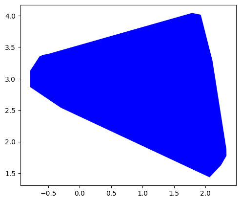
[7]:
whole_tree_hull,_ = myCollection.watershed_boundary(
plane="XY",
curvature_alpha=0.15,
draw=True,
)
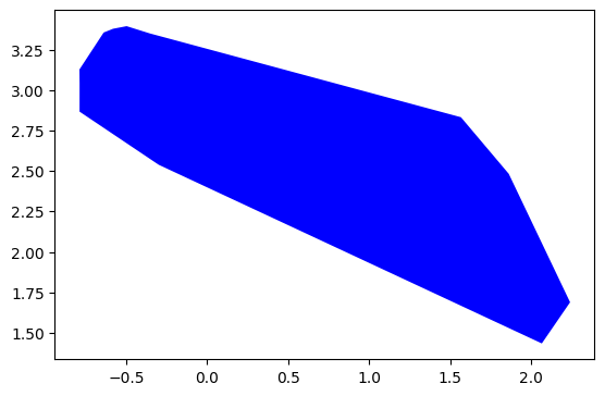
# plotting the boundary of the stemflow generating portion alone
stem_flow_hull,_ = myCollection.watershed_boundary(
plane="XY",
curvature_alpha=0.15,
filter_lambda=lambda: is_stem ,
draw=True,
)
2024.10.14 21:19:27.690 |MainThread | INFO | geometry.py:563 - draw_cyls() | model - Plotting cylinder collection
2024.10.14 21:19:27.904 |MainThread | INFO | geometry.py:563 - draw_cyls() | model - Plotting cylinder collection
In doing so, we can calculate statistics for only the subset of cylinders that contribute to stemflow.
[8]:
# Demonstrating how statistics can be generated from hul objects
print(type(stem_flow_hull))

print('Whole Tree Coverage Area:')
print(whole_tree_hull.area)

print('Stem Flow Coverage Area:')
print(stem_flow_hull.area)


print('')

print('Whole Tree Coverage Bounds:')
print(whole_tree_hull.bounds)

print('Stem Flow Coverage Bounds:')
print(stem_flow_hull.bounds)

print('')

# Demonstrating how is_stem might be used in other calculations
total_volume= np.sum([cyl.volume
                                for cyl in myCollection.cylinders
                                if cyl.is_stem]
                        )
<class 'shapely.geometry.polygon.Polygon'>
Whole Tree Coverage Area:
4.828740395823999
Stem Flow Coverage Area:
2.66555606734

Whole Tree Coverage Bounds:
(-0.788937, 1.434109, 2.336527, 4.043691)
Stem Flow Coverage Bounds:
(-0.788937, 1.434109, 2.241708, 3.394286)
For detailed definitions of all of the statistics availible to users, see the Glossary